UI /

TrackingProblem

Tracking problem

Tracking of time varying references
Tracking with delta u formulation
Tracking with builtin integrator

Tracking of time varying references

State tracking

Consider an LTI system with 3 states and 2 inputs subject to state and input constraints

model = LTISystem('A', [ -0.79 -0.3 -0.1; 0.5 0.82 1.23; 0.52 -0.3 -0.5], 'B', [ -2.04 -0.21; -1.28 2.75; 0.29 -1.41]);
model.x.min = [-10; -9; -8];
model.x.max = [10; 9; 8];
model.u.min = [-2; -3];
model.u.max = [2; 3];

The objective is to track the second state that varies in time. To provide a time-varying reference the reference filter is activated on the state signal and the value is set to "free", indicating a time-varying reference.

model.x.with('reference');
model.x.reference = 'free';

In the remainder of the MPC setup, the penalties on the states and inputs are provided.

model.x.penalty = OneNormFunction( diag([0.5, 1, 0]) );
model.u.penalty = OneNormFunction( eye(2) );

and the online MPCController object is constructed with horizon 4:

ctrl = MPCController(model, 4)

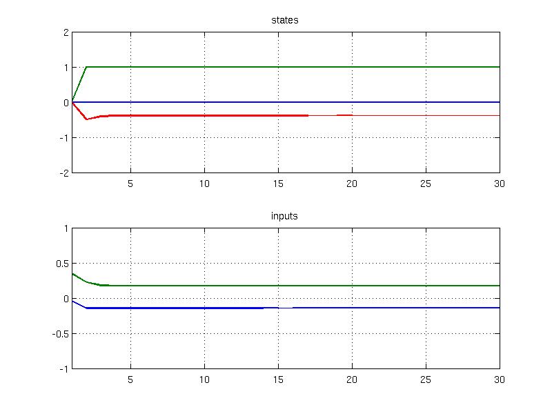
For simulation purposes, a closed loop object is constructed and simulated for a constant reference value [0; 1; 0] over 30 samples

loop = ClosedLoop(ctrl, model);
x0 = [0; 0; 0];
Nsim = 30;
xref = [0; 1; 0];
data = loop.simulate(x0, Nsim, 'x.reference', xref)

The results of the simulation can be plotted nicely

subplot(2, 1, 1);
plot(1:Nsim, data.X(:,1:Nsim), 'linewidth', 2);
axis([1, Nsim, -2, 2]);
grid on; title('states');
subplot(2, 1, 2); plot(1:Nsim, data.U, 'linewidth', 2);
axis([1, Nsim, -1, 1]);
grid on; title('inputs');

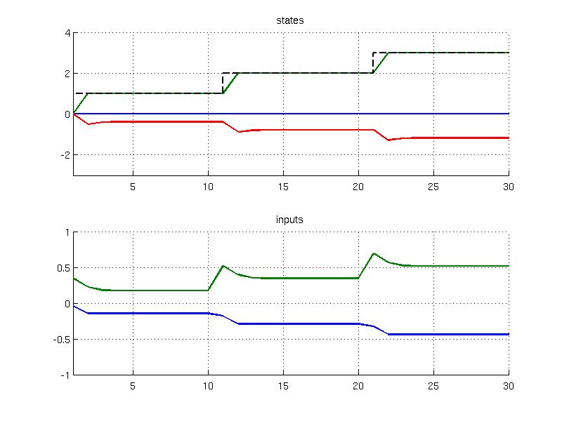
The simulate method also allows to provide time-varying profiles of references, e.g.

xref1 = [0; 1; 0];
xref2 = [0; 2; 0];
xref3 = [0; 3; 0];
xref = [repmat(xref1, 1, 10), repmat(xref2, 1, 10), repmat(xref3, 1, 10)];
x0 = [0; 0; 0];
Nsim = 30;
data = loop.simulate(x0, Nsim, 'x.reference', xref);
subplot(2, 1, 1); hold on; grid on;
plot(1:Nsim, data.X(:,1:Nsim), 'linewidth', 2);
stairs(1:Nsim, xref(2,:), 'k--', 'linewidth', 2);
axis([1, Nsim, -3, 4]);
title('states')
subplot(2, 1, 2); hold on; grid on;
plot(1:Nsim, data.U, 'linewidth', 2);
axis([1, Nsim, -1, 1]);
title('inputs')

The same result can be obtained manually using a for-loop as follows:

x0 = zeros(3,1);
X = []; U = [];
model.initialize(x0);
for i=1:30
X = [X, x0];
if i<10
xref = [0; 1; 0];
elseif i<20
xref = [0; 2; 0];
else
xref = [0; 3; 0];
end
u = ctrl.evaluate(x0, 'x.reference', xref);
U = [U, u];
x0 = model.update(u);
end
subplot(2,1,1); plot(1:30,X); title('states')
subplot(2,1,2); plot(1:30,U); title('inputs')

Output tracking

Consider a simple PWA system that comprises of two modes and has one output

mode1 = LTISystem('A', [ 0.4 0.69; -0.69 0.4], 'B', [0;1], 'C', [1, 0]);
mode1.setDomain('x', Polyhedron('A', [1 0], 'b', 0) );
mode2 = LTISystem('A', [ 0.4 -0.69; 0.69 0.4], 'B', [0;1], 'C', [1, 0]);
mode2.setDomain('x', Polyhedron('A', [-1 0], 'b', 0) );
model = PWASystem([mode1, mode2]);

The model is subject to input/output constraints

model.u.min = -3;
model.u.max = 3;
model.y.min = -10;
model.y.max = 10;

The objective is to track the time varying output while satisfying the constraints. To incorporate a time varying signal one needs to active the appropriate reference filter and mark it as "free"

model.y.with('reference');
model.y.reference = 'free';

To finalize the MPC setup, penalty on inputs and outputs are provided

model.y.penalty = OneNormFunction( 3 );
model.u.penalty = OneNormFunction( 0.5 );

and the online MPCController object is constructed with horizon 3

ctrl = MPCController(model, 3);

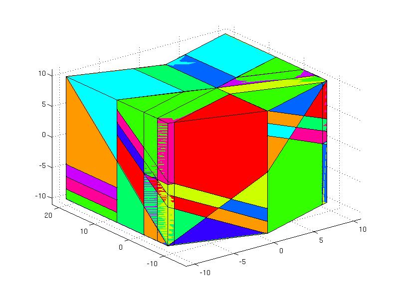
After testing the performance of the online-controller, one can export it to the explicit form as follows:

ectrl = ctrl.toExplicit();

and plot the partition

ectrl.partition.plot()

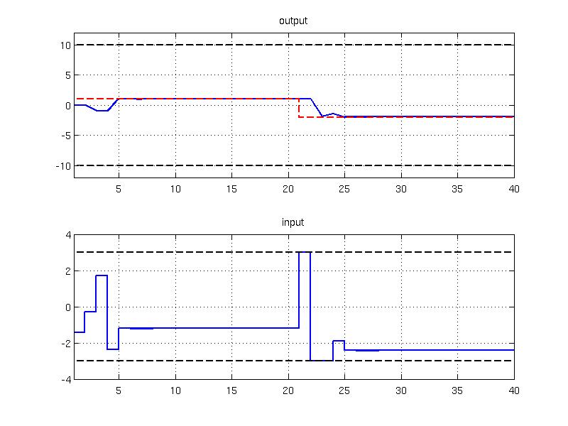
The closed-loop simulation can be evaluated using the ClosedLoop object

loop = ClosedLoop(ectrl, model);

by providing the time varying reference signal yref

yref1 = 1;
yref2 = -2;
yref = [repmat(yref1, 1, 20), repmat(yref2, 1, 20)];
x0 = zeros(2,1);
Nsim = 40;
data = loop.simulate(x0, Nsim, 'y.reference', yref);

The simulation results are stored in the output variable data and can be plotted

subplot(2, 1, 1); plot(1:Nsim, data.Y, 'linewidth', 2);
hold on; grid on;
plot(1:Nsim, model.y.max*ones(1, Nsim), 'k--', 'linewidth', 2);
plot(1:Nsim, model.y.min*ones(1, Nsim), 'k--', 'linewidth', 2);
stairs(1:Nsim, yref, 'r--', 'linewidth', 2);
axis([1, Nsim, -12, 12]);
title('output')
subplot(2, 1, 2); stairs(1:Nsim, data.U, 'linewidth', 2);
hold on; grid on;
plot(1:Nsim, model.u.max*ones(1, Nsim), 'k--', 'linewidth', 2);
plot(1:Nsim, model.u.min*ones(1, Nsim), 'k--', 'linewidth', 2);
axis([1, Nsim, -4, 4]);
title('input')

In the next code sample you can find the manual decomposition of the simulation which shows the step-wise changes in the output reference over 30 samples and the input is obtained by evaluating the explicit controller

x0 = zeros(2,1);
Y = []; U = [];
model.initialize(x0);
for i=1:40
if i<20
yref = 1;
else
yref = -2;
end
u = ectrl.evaluate(x0, 'y.reference', yref);
U = [U, u];
[x0, y] = model.update(u);
Y = [Y, y];
end
subplot(2, 1, 1); plot(1:40, Y); title('output')
subplot(2, 1, 2); stairs(1:40, U); title('input')

Tracking with delta u formulation

Consider the following unstable LTI system subject to input and state constraints

model = LTISystem('A', 1.5 , 'B', 1);
model.x.min = -10;
model.x.max = 10;
model.u.min = -5;
model.u.max = 5;

The objective is to follow a time-varying state signal subject to delta-u formulation. The activation of the time-varying signal is achived via "reference" filter

model.x.with('reference');
model.x.reference = 'free';
model.x.penalty = QuadFunction(5);

The delta-u formulation {$ \Delta u_k = u_k - u_{k-1} $} is activated with the "deltaPenalty" filter

model.u.with('deltaPenalty');
model.u.deltaPenalty = QuadFunction(1);

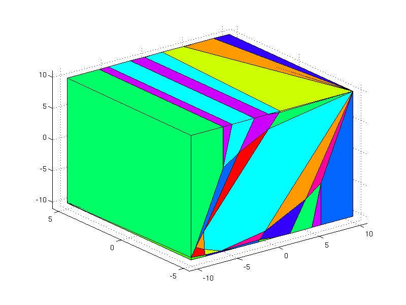
The online MPCController object is created with a horizon 4 and exported to an explicit form

ctrl = MPCController(model, 4);
ectrl = ctrl.toExplicit();

Note that the partition of the explicit controller is defined in dimension three because the parametric variable is the current state {$x_k$}, the previous value of the input {$u_{k-1}$}, and the reference signal {$ r_k $}. This can be verified by plotting the partition of the controller

ectrl.partition.plot()

For simulation purposes, the ClosedLoop object is created with the explicit controller and the same model that was used for MPC design

loop = ClosedLoop( ectrl, model);

Simulate the performance of the explicit controller in 20 samples

x0 = 0;
u0 = 0;
xref1 = 5;
xref2 = -3;
Nsim = 20;
xref = [repmat( xref1, 1, Nsim/2), repmat(xref2, 1, Nsim/2)];
data = loop.simulate(x0, Nsim, 'u.previous', u0, 'x.reference', xref);

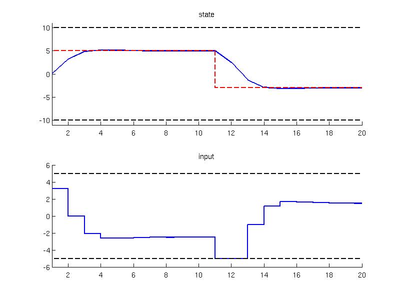
and plot the closed loop trajectories

subplot(2, 1, 1); hold on;
plot(1:Nsim, data.X(1:Nsim), 'linewidth', 2 );
plot(1:Nsim, model.x.max*ones(1,Nsim), 'k--', 'linewidth', 2);
plot(1:Nsim, model.x.min*ones(1,Nsim), 'k--', 'linewidth', 2);
stairs(1:Nsim, xref, 'r--', 'linewidth', 2);
axis([1, Nsim, -11, 11]);
title('state')
subplot(2, 1, 2); hold on;
stairs(1:Nsim, data.U, 'linewidth', 2);
plot(1:Nsim, model.u.max*ones(1, Nsim), 'k--', 'linewidth', 2);
plot(1:Nsim, model.u.min*ones(1, Nsim), 'k--', 'linewidth', 2);
axis([1, Nsim, -6, 6]);
title('input')

Tracking with builtin integrator

The tracking of a time-varying reference can be achieved by augmenting the state with an integrator state that predicts the steady state values. In MPT this can be achieved with the help of "integrator" filter that extends the model with an integrator state. Consider the unstable LTI system as in the previous example that operates under input and state constraints

model = LTISystem('A', 1.5 , 'B', 1 );
model.x.min = -10;
model.x.max = 10;
model.u.min = -5;
model.u.max = 5;

Activate the time-varying reference

model.x.with('reference');
model.x.reference = 'free';

To add the integrator, one need to active the "integrator" filter as follows.

model.with('integrator');

In the remainder of MPC set, the penalty on the predicted difference of the integrator state and the reference is provided

model.x.penalty = QuadFunction( 5 );

as well as the penalty on the inputs

model.u.penalty = QuadFunction( 1 );

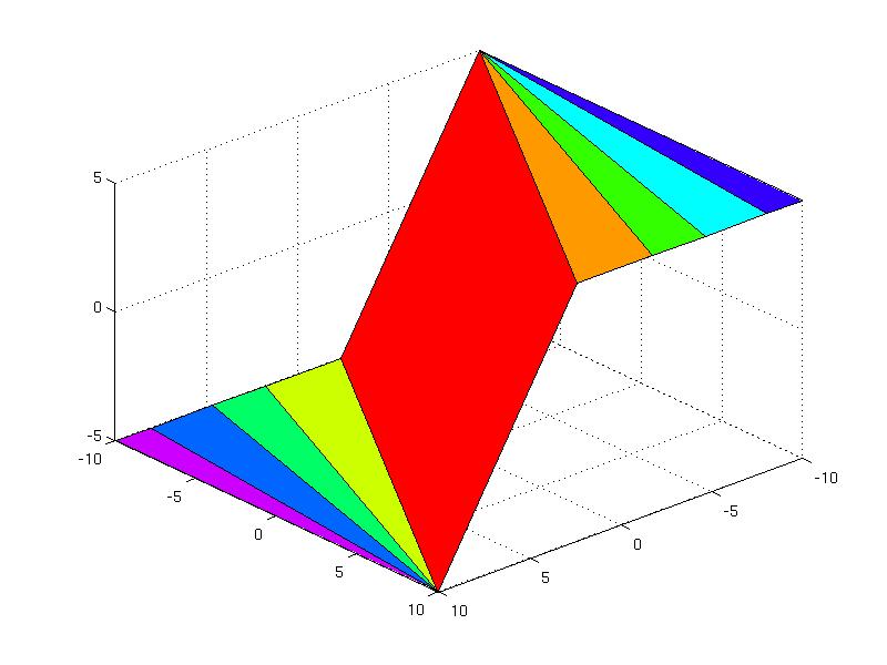
The resulting controller is exported to an explicit form

ctrl = MPCController(model, 4);
ectrl = ctrl.toExplicit();

and can be plotted with the help of fplot function

ectrl.feedback.fplot()

In the next step, the explicit controller is employed in the closed loop object

loop = ClosedLoop( ectrl, model);

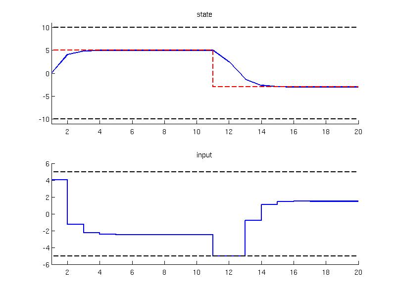
The simulation results are the same as in the previous example, but this time obtained with the integrator state

x0 = 0;
u0 = 0;
xref1 = 5;
xref2 = -3;
Nsim = 20;
xref = [repmat( xref1, 1, Nsim/2), repmat(xref2, 1, Nsim/2)];
data = loop.simulate(x0, Nsim, 'u.previous', u0, 'x.reference', xref);

The simulated data can be plotted together with the reference signal and constraints

Back to MPC synthesis overview.