RegulationProblem
UI.RegulationProblem History
Hide minor edits - Show changes to markup
Regulation problem
Regulation problem
Finite horizon MPC
Finite horizon MPC
Online solution
Explicit solution
Finite horizon MPC with terminal penalty and terminal set constraints
Finite horizon MPC with terminal penalty and terminal set constraints
Regulation to a nonzero steady state
Regulation to a nonzero steady state
As an example, let us consider an LTI prediction model, represented by the state-update equation x^+ = A x + B u with A = [1 1; 0 1] and B = [1; 0.5]:
As an example, let us consider an LTI prediction model, represented by the state-update equation {$x^+ = A x + B u$} with {$A = \begin{bmatrix} 1 & 1 \\ 0 & 1 \end{bmatrix}$} and {$ B = \begin{bmatrix} 1 \\ 0.5 \end{bmatrix} $}
- Add state constraints
[-5; -5] <= x <= [5; 5]:
- Add state constraints {$ \begin{bmatrix} -5 \\ -5 \end{bmatrix} \le x \le \begin{bmatrix} 5 \\ 5 \end{bmatrix} $}
- Add input constraints
-1 <= u <= 1:
- Add input constraints {$-1 \le u \le 1 $}:
- Add quadratic state penalty, i.e., penalize
x_k^T Q x_kwithQ = [1 0; 0 1]:
- Add quadratic state penalty, i.e., penalize {$ x_k^T Q x_k $} with {$ Q = \begin{bmatrix} 1 & 0 \\ 0 & 1 \end{bmatrix} $}
- Use quadratic penalization of inputs, i.e.,
u_k^T R u_kwithR=1:
- Use quadratic penalization of inputs, i.e., {$ u_k^T R u_k $} with {$ R=1 $}:
Finally, we can synthesize an MPC controller with prediction horizon say N=5:
Finally, we can synthesize an MPC controller with prediction horizon say {$ N=5 $}:
As an example, let use consider an LTI prediction model, represented by the state-update equation x^+ = A x + B u with A = [1 1; 0 1] and B = [1; 0.5]:
As an example, let us consider an LTI prediction model, represented by the state-update equation x^+ = A x + B u with A = [1 1; 0 1] and B = [1; 0.5]:
model.u.penalty = OneFunction(R);
model.u.penalty = QuadFunction(R);
Regulation to nonzero steady state
Regulation to a nonzero steady state
Regulation to nonzero steady state
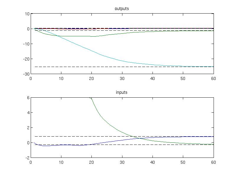
The next example demonstrates how to achieve regulation to a nonzero steady state. Consider a model of an aircraft discretized with 0.2s sampling time
(:source lang=MATLAB -getcode:)
A = [0.99 0.01 0.18 -0.09 0; 0 0.94 0 0.29 0; 0 0.14 0.81 -0.9 0; 0 -0.2 0 0.95 0; 0 0.09 0 0 0.9];
B = [0.01  -0.02; -0.14 0; 0.05 -0.2; 0.02 0; -0.01 0];
C = [0 1 0 0 -1; 0 0 1 0 0; 0 0 0 1 0; 1 0 0 0 0];
model = LTISystem('A', A, 'B', B, 'C', C, 'Ts', 0.2);
Given the dynamics of the model, one can compute the new steady state values for a particular value of the input, e.g.
(:source lang=MATLAB -getcode:)us = [0.8; -0.3]; ys = C*( (eye(5)-A)\B*us );
The computed values will be used as references for the desired steady state which can be added using "reference" filter
(:source lang=MATLAB -getcode:)
model.u.with('reference');
model.u.reference = us;
model.y.with('reference');
model.y.reference = ys;
To fomulate MPC optimization problem one shall provide constraints and penalties on the system signals. In this example, only the input constraints are considered
(:source lang=MATLAB -getcode:)model.u.min = [-5; -6]; model.u.max = [5; 6];
The penalties on outputs and inputs are provided as quadratic functions
(:source lang=MATLAB -getcode:)model.u.penalty = QuadFunction( diag([3, 2]) ); model.y.penalty = QuadFunction( diag([10, 10, 10, 10]) );
which yields a quadratic optimization problem to be solved in MPC. The online MPC controller object is constructed with a horizon 6
(:source lang=MATLAB -getcode:)ctrl = MPCController(model, 6)
and simulated for zero initial conditions over 30 samples
(:source lang=MATLAB -getcode:)loop = ClosedLoop(ctrl, model); x0 = [0; 0; 0; 0; 0]; Nsim = 30; data = loop.simulate(x0, Nsim);
The simulation results can be plotted to inspect that the convergence to the new steady state has been achieved
(:source lang=MATLAB -getcode:)
subplot(2,1,1)
plot(1:Nsim, data.Y);
hold on;
plot(1:Nsim, ys*ones(1, Nsim), 'k--')
title('outputs')
subplot(2,1,2)
plot(1:Nsim, data.U);
hold on;
plot(1:Nsim, us*ones(1, Nsim), 'k--')
title('inputs')
Finite horizon MPC
h1. Adding terminal set and terminal penalty
Regulation problem
To create an MPC controller in MPT3, use the MPCController constructor:
mpc = MPCController(sys)
where sys represents the prediction model, created by LTISystem, PWASystem or MLDSystem constructors (see here).
As an example, let use consider an LTI prediction model, represented by the state-update equation x^+ = A x + B u with A = [1 1; 0 1] and B = [1; 0.5]:
model = LTISystem('A', [1 1; 0 1], 'B', [1; 0.5]);
Next we specify more properties of the model:
- Add state constraints
[-5; -5] <= x <= [5; 5]:
model.x.min = [-5; -5];
model.x.max = [5; 5];
- Add input constraints
-1 <= u <= 1:
model.u.min = -1;
model.u.max = 1;
- Add quadratic state penalty, i.e., penalize
x_k^T Q x_kwithQ = [1 0; 0 1]:
Q = [1 0; 0 1];
model.x.penalty = QuadFunction(Q);
- Use quadratic penalization of inputs, i.e.,
u_k^T R u_kwithR=1:
R = 1;
model.u.penalty = OneFunction(R);
A number of other constraints and penalties can be added using the concept of filters.
Finally, we can synthesize an MPC controller with prediction horizon say N=5:
N = 5;
mpc = MPCController(model, N)
Now the mpc object is ready to be used as an MPC controller. For instance, we can ask it for the optimal control input for a given value of the initial state:
x0 = [4; 0];
u = mpc.evaluate(x0)

u =

    -1
You can also retrieve the full open-loop predictions:
(:source lang=MATLAB -getcode:)
[u, feasible, openloop] = mpc.evaluate(x0)

openloop =

    cost: 32.4898
       U: [-1 -1 0.1393 0.3361 -5.2042e-16]
       X: [2x6 double]
       Y: [0x5 double]
Please consult this page to learn how to perform closed-loop simulations in MPT3.
Once you are satisfied with the controller's performance, you can convert it to an explicit form by calling the toExplicit() method:
expmpc = mpc.toExplicit();
This will generate an instance of the EMPCController class, which represents all explicit MPC controllers in MPT3. Explicit controllers can be used for evaluation/simulation in exactly the same way, i.e.,
[u, feasible, openloop] = expmpc.evaluate(x0)

openloop =

    cost: 32.4898
       U: [-1 -1 0.1393 0.3361 -5.2042e-16]
       X: [2x6 double]
       Y: [0x5 double]
h1. Adding terminal set and terminal penalty
Consider an oscillator model defined in 2D.
(:source lang=MATLAB -getcode:)A = [ 0.5403, -0.8415; 0.8415, 0.5403]; B = [ -0.4597; 0.8415]; C = [1 0]; D = 0;
Linear discrete-time model with sample time 1
(:source lang=MATLAB -getcode:)sys = ss(A,B,C,D,1); model = LTISystem(sys);
Set constraints on output
(:source lang=MATLAB -getcode:)model.y.min = -10; model.y.max = 10;
Set constraints on input
(:source lang=MATLAB -getcode:)model.u.min = -1; model.u.max = 1;
Include weights on states/inputs
(:source lang=MATLAB -getcode:)model.x.penalty = QuadFunction(eye(2)); model.u.penalty = QuadFunction(1);
Compute terminal set
(:source lang=MATLAB -getcode:)Tset = model.LQRSet;
Compute terminal weight
(:source lang=MATLAB -getcode:)PN = model.LQRPenalty;
Add terminal set and terminal penalty
(:source lang=MATLAB -getcode:)
model.x.with('terminalSet');
model.x.terminalSet = Tset;
model.x.with('terminalPenalty');
model.x.terminalPenalty = PN;
Formulate finite horizon MPC problem
(:source lang=MATLAB -getcode:)ctrl = MPCController(model,5);