RegulationProblem
Regulation problem
- Finite horizon MPC
- Finite horizon MPC with terminal penalty and terminal set constraints
- Regulation to a nonzero steady state
Finite horizon MPC
To create an MPC controller in MPT3, use the MPCController constructor:
where sys represents the prediction model, created by LTISystem, PWASystem or MLDSystem constructors (see here).
As an example, let us consider an LTI prediction model, represented by the state-update equation {$x^+ = A x + B u$} with {$A = \begin{bmatrix} 1 & 1 \\ 0 & 1 \end{bmatrix}$} and {$ B = \begin{bmatrix} 1 \\ 0.5 \end{bmatrix} $}
Next we specify more properties of the model:
- Add state constraints {$ \begin{bmatrix} -5 \\ -5 \end{bmatrix} \le x \le \begin{bmatrix} 5 \\ 5 \end{bmatrix} $}
model.x.max = [5; 5];
- Add input constraints {$-1 \le u \le 1 $}:
model.u.max = 1;
- Add quadratic state penalty, i.e., penalize {$ x_k^T Q x_k $} with {$ Q = \begin{bmatrix} 1 & 0 \\ 0 & 1 \end{bmatrix} $}
model.x.penalty = QuadFunction(Q);
- Use quadratic penalization of inputs, i.e., {$ u_k^T R u_k $} with {$ R=1 $}:
model.u.penalty = QuadFunction(R);
A number of other constraints and penalties can be added using the concept of filters.
Online solution
Finally, we can synthesize an MPC controller with prediction horizon say {$ N=5 $}:
mpc = MPCController(model, N)
Now the mpc object is ready to be used as an MPC controller. For instance, we can ask it for the optimal control input for a given value of the initial state:
u = mpc.evaluate(x0)
u =
-1
You can also retrieve the full open-loop predictions:
openloop =
cost: 32.4898
U: [-1 -1 0.1393 0.3361 -5.2042e-16]
X: [2x6 double]
Y: [0x5 double]
Please consult this page to learn how to perform closed-loop simulations in MPT3.
Explicit solution
Once you are satisfied with the controller's performance, you can convert it to an explicit form by calling the toExplicit() method:
This will generate an instance of the EMPCController class, which represents all explicit MPC controllers in MPT3. Explicit controllers can be used for evaluation/simulation in exactly the same way, i.e.,
openloop =
cost: 32.4898
U: [-1 -1 0.1393 0.3361 -5.2042e-16]
X: [2x6 double]
Y: [0x5 double]
Finite horizon MPC with terminal penalty and terminal set constraints
Consider an oscillator model defined in 2D.
B = [ -0.4597; 0.8415];
C = [1 0];
D = 0;
Linear discrete-time model with sample time 1
model = LTISystem(sys);
Set constraints on output
model.y.max = 10;
Set constraints on input
model.u.max = 1;
Include weights on states/inputs
model.u.penalty = QuadFunction(1);
Compute terminal set
Compute terminal weight
Add terminal set and terminal penalty
model.x.terminalSet = Tset;
model.x.with('terminalPenalty');
model.x.terminalPenalty = PN;
Formulate finite horizon MPC problem
Regulation to a nonzero steady state
The next example demonstrates how to achieve regulation to a nonzero steady state. Consider a model of an aircraft discretized with 0.2s sampling time
B = [0.01 -0.02; -0.14 0; 0.05 -0.2; 0.02 0; -0.01 0];
C = [0 1 0 0 -1; 0 0 1 0 0; 0 0 0 1 0; 1 0 0 0 0];
model = LTISystem('A', A, 'B', B, 'C', C, 'Ts', 0.2);
Given the dynamics of the model, one can compute the new steady state values for a particular value of the input, e.g.
ys = C*( (eye(5)-A)\B*us );
The computed values will be used as references for the desired steady state which can be added using "reference" filter
model.u.reference = us;
model.y.with('reference');
model.y.reference = ys;
To fomulate MPC optimization problem one shall provide constraints and penalties on the system signals. In this example, only the input constraints are considered
model.u.max = [5; 6];
The penalties on outputs and inputs are provided as quadratic functions
model.y.penalty = QuadFunction( diag([10, 10, 10, 10]) );
which yields a quadratic optimization problem to be solved in MPC. The online MPC controller object is constructed with a horizon 6
and simulated for zero initial conditions over 30 samples
x0 = [0; 0; 0; 0; 0];
Nsim = 30;
data = loop.simulate(x0, Nsim);
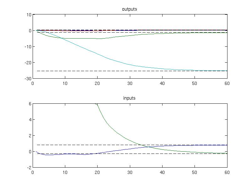
The simulation results can be plotted to inspect that the convergence to the new steady state has been achieved
plot(1:Nsim, data.Y);
hold on;
plot(1:Nsim, ys*ones(1, Nsim), 'k--')
title('outputs')
subplot(2,1,2)
plot(1:Nsim, data.U);
hold on;
plot(1:Nsim, us*ones(1, Nsim), 'k--')
title('inputs')
Back to MPC synthesis overview.