stairs(1:Nsim, data.U, 'linewidth', 2); hold on;

model.u.min = -2; model.u.max = 2;

The finite horizon optimal control problem is constructed with the prediction {$ N=4 $} by constructing the MPCController object

ctrl = MPCController(model, 4);

The simulation of a closed loop system is performed over 10 samples

loop = ClosedLoop(ctrl, model);
Nsim = 10;
x0 = [0; 0; 0];
data = loop.simulate(x0, Nsim)

and plotted

subplot(2, 1, 1); 
plot(1:Nsim, data.Y, 'linewidth', 2); hold on;
plot(1:Nsim, 2*ones(1,Nsim), 'k--', 'linewidth', 2);
axis([1, Nsim, -3, 3]);
title('output');
subplot(2, 1, 2);
plot(1:Nsim, data.U, 'linewidth', 2); hold on;
plot(1:Nsim, 2*ones(1,Nsim), 'k--', 'linewidth', 2);
plot(1:Nsim, -2*ones(1,Nsim), 'k--', 'linewidth', 2);
axis([1, Nsim, -3, 3]);
title('input'); 

• Reference signal - reference

Reference signal

The system model used in MPC synthesis can be extended with reference signals by activating the reference filter. If activated, the difference of the current signal {$s$} versus the given reference {$r$} is going to be penalized, i.e. {$ s - r $}. The value for the reference signal can be be constant, or time-varying. In the case of time varying signal, it is marked with a string as 'free'. For more details on design with time-varying references, see the part on MPC tracking problems. In the next example, a penalization to constant, non-zero reference is shown. The model is described with one input, one output and three states as follows

A = [1.45  -0.85 0.29; 1 0 0; 0 0.25 0];
B = [1; 0; 0];
C = [0.41 0.28 -0.19];
model = LTISystem('A', A, 'B', B, 'C', C, 'Ts', 1);

The input signal is constrained

model.u.min = -1;
model.u.max = 1;

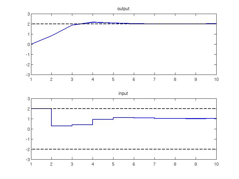
The objective of the MPC design is to minimize the quadratic cost function {$ \sum_{k=0}^{N-1} ( u_{k}^{T}Ru_{k} + (y_{k}-r)^{T}Q(y_{k}-r) ) $} by steering the output to the reference value {$r = 2$}. In MPT this can be achieved by providing the corresponding penalties on the signals

R = 1;
model.u.penalty = QuadFunction( R );
Q = 5;
model.y.penalty = QuadFunction( Q );
r = 2;
model.y.with('reference');
model.y.reference = r;

• Penalty on the terminal state - terminalPenalty

The new MPC controller object is created and exported to explicit form

The closed loop simulation is invoked and tested for multiple initial conditions

ectrl_new.clicksim()

The explicit controller ectrl_new designed with the terminal penalty and terminal set constraint is defined over smaller feasible area than ectrl but is able to stabilize the closed loop system for all initial conditions inside the feasible area.

To remedy the stabilizing properties of the controller, the terminal penalty and the terminal set constraint are computed with the help of LQRPenalty and LQRSet methods

P = model.LQRPenalty; Tset = model.LQRSet;

Subsequently, the appropriate filters are activated

model.x.with('terminalPenalty');

and the corresponding values are provided

• Signal rate penalization - terminalPenalty

Terminal penalty

The terminalPenalty filter activates penalization of the state variables at the end of the prediciton horizon. In general, the terminal penalty function can be artibrary but for stability reasons it is often required that the terminal penalty satisfies certain properties. Typically, the terminal penalty is often computed as a value function of an unconstrained infinite horizon optimal control problem which has associated a stabilizing controller. Consider a stable linear system subject to convex constraints

 model = LTISystem('A', [-1.08 -1.52; 0.2 -0.72], 'B', [0.03; 0.55]);
 model.x.min = [-10; -9];
 model.x.max = [10; 9];
 model.u.min = -2;
 model.u.max = 2;

The objective is to regulate the system to the origin by means of MPC. The performance criterion is a quadratic function with weighing factors {$ Q = I $} and {$ R = 0.1 $}

Q = eye(2);
model.x.penalty = QuadFunction( Q );
R = 0.1;
model.u.penalty = QuadFunction( R );

The finite horizon MPC controller is defined over the horizon 2 and exported to explicit form

 ctrl = MPCController(model, 2)
 ectrl = ctrl.toExplicit()

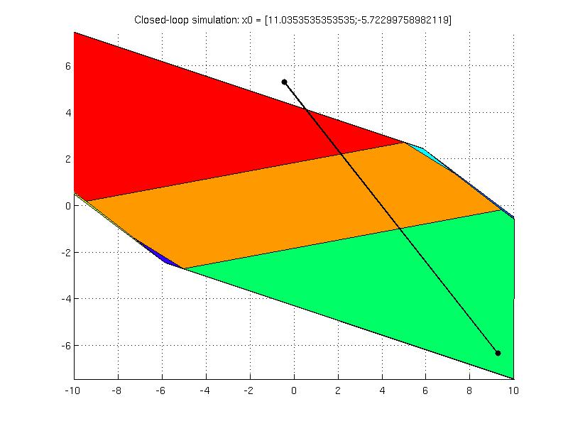
The animated simulation for one initial condition reveals that the controller does not provide stabilizing feedback

 ectrl.clicksim()

To remedy the stabilizing properties of the controller, the terminal penalty is included to the model by activating the terminalPenalty filter

model.x.with('terminalPenalty');

together with the terminal set constraint

model.x.with('terminalSet');

The values of the terminal set and penalty are computed with the help of LQRPenalty and LQRSet methods

P = model.LQRPenalty;
Tset = model.LQRSet;
model.x.terminalPenalty = P;
model.x.terminalSet = Tset;

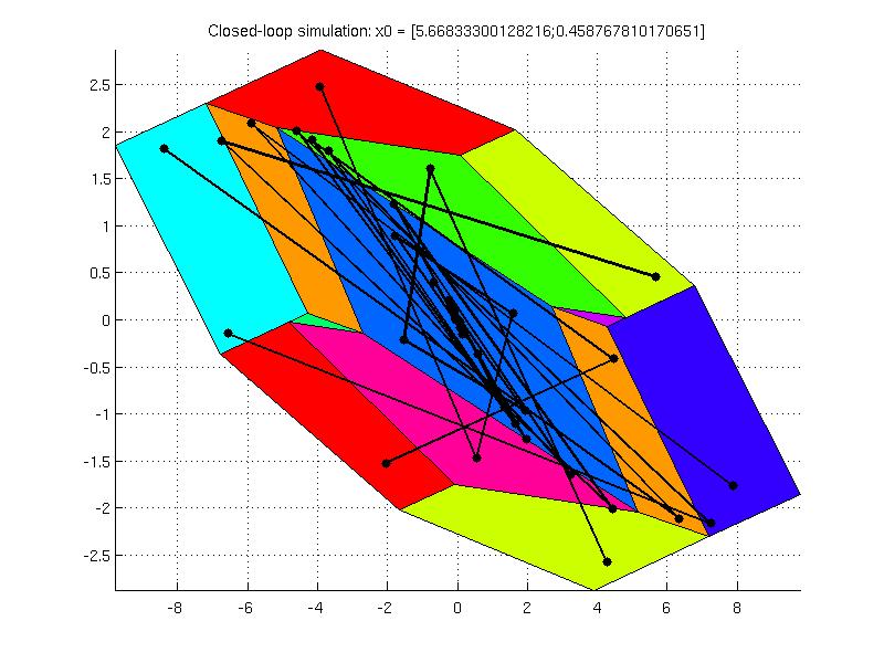
The new MPC controller object is created and simulated again

 ctrl_new = MPCController(model, 2)
 ectrl_new = ctrl_new.toExplicit()

The new controller designed with the terminal penalty and terminal set constraint is able to stabilize the system for multiple condtions as is evident from the figure below. (:comment However, the presence of the terminal set/terminal constraint resulted in a controller that is defined over smaller feasible area as before because the unstable parts have been removed. :)

• Binary constraint - binary
• Move blocking constraint - block
• Initial set constraint - initialSet
• Set constraint - setConstraint
• Terminal set constraint - terminalSet

(:comment ** [[#terminalController | Terminal controller - @@terminalController@@]] :)

• Upper bound limit on a signal - max
• Lower bound limit on a signal - min
• Upper bound limit on a rate of a signal - deltaMax
• Lower bound limit on a rate of a signal - deltaMin
• Soft upper bound constraint - softMax
• Soft lower bound constraint - softMin

• Signal rate penalization - deltaPenalty

(:comment ** [[#terminalPenalty | Signal rate penalization - @@terminalPenalty@@ ]] :) (:comment ** [[#reference | Reference signal - @@reference@@ ]] :) (:comment ** [[#PWApenalty | Piecewise Affine penalty - @@PWApenalty@@ ]] :)

(:comment ** [[#terminalController | Terminal controller -- @@terminalController@@]] :)

(:comment ** [[#terminalPenalty | Signal rate penalization -- @@terminalPenalty@@ ]] :) (:comment ** [[#reference | Reference signal -- @@reference@@ ]] :) (:comment ** [[#PWApenalty | Piecewise Affine penalty -- @@PWApenalty@@ ]] :)

(:comment [[#terminalController]] !!! Terminal Controller :)

(:comment [[#terminalPenalty]] !!! Terminal penalty :)

(:comment [[#reference]] !!! Reference signal :)

(:comment [[#PWApenalty]] !!! Piecewise Affine penalty :)

• Terminal controller -- terminalController

TODO.

TODO.

TODO.

TODO.

@] The results of the simulation are plotted in the figure below with the constraints depicted with dashed lines (:source lang=MATLAB -getcode:) [@

hold on plot(1:Nsim, model.x.min*ones(1,Nsim), 'k--', 1:Nsim, model.x.max*ones(1,Nsim), 'k--'); axis([1 Nsim -12 12]);

hold on plot(1:Nsim, model.u.min*ones(1,Nsim), 'k--', 1:Nsim, model.u.max*ones(1,Nsim), 'k--'); axis([1 Nsim -1.2 1.2]);

• Terminal controller -- terminalController@

One can observe that the desired terminal state has been achieved in five steps of the prediction.

Terminal Controller

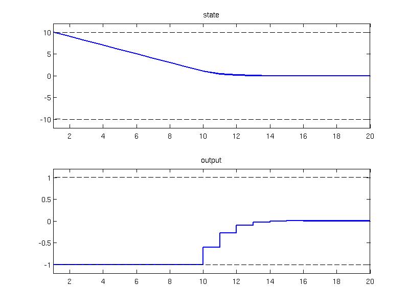
It is sometimes of interest to add penalization on the rate of the signal {$\Delta s_k = s_k - s_{k-1} $}. This can be achieved by activating the filter deltaPenalty and specifying the penalty function. As an example, consider the simple model {$ x_{k+1} = x_{k} + u_{k} $}

model = LTISystem('A', 1, 'B', 1);

subject to input and state constraints

model.x.min = -10;
model.x.max = 10;
model.u.min = -1;
model.u.max = 1;

The objective is to regulate the system by minimizing the quadratic optimization criterion {$ \sum_{k=0}^{N-1} (x_{k}^{T}Qx_k + u_k^{T}Ru_k + \Delta u_k^TS\Delta u_k) $}. To activate the penalty on the input rate the filter deltaPenalty is provided:

Q = 1;
R = 1;
S = 1;
model.x.penalty = QuadFunction( Q );
model.u.penalty = QuadFunction( R );
model.u.with('deltaPenalty');
model.u.deltaPenalty = QuadFunction( S );

The MPCController object is constructed with horizon 5 and exported to explicit form

ctrl = MPCController( model, 5);
explicit_ctrl = ctrl.toExplicit();

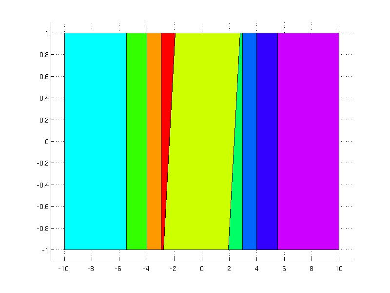
Since the deltaPenalty is activated, the explicit controller is designed for the augmented system where the previous value of the input is the second state variable. The explicit controller can be plotted

explicit_ctrl.partition.plot

and simulated in the closed loop setting for the initial condition x0 = 10, u0 = 0

loop = ClosedLoop(explicit_ctrl, model);
x0 = 10; u0 = 0; 
Nsim = 20;
data = loop.simulate(x0, Nsim, 'u.previous', u0);
subplot(2, 1, 1); plot(1:Nsim, data.X(1:Nsim), 'linewidth', 2); title('state');
subplot(2, 1, 2); stairs(1:Nsim, data.U, 'linewidth', 2); title('output');

Terminal penalty

Note that the reference for the output signal {$y=1$} lies close to the upper {$ 0\le y_k \le 1.2 $} which could be potentially violated with external disturbances.

{$$ G(s) = \frac{2} {s^2 + 2s + 1} $$}

continuous_model = tf(2, [1 2 1]);

In order to model the external disturbance, the closed loop simulation is performed manually over 20 instances and the external disturbance is added at the 10th sample:

Nsim = 20;
x0 = [0;0];
Y = []; U = [];
model.initialize(x0);
for i=1:Nsim
   if i==10
      x0 = x0 + [-1.6; 0.9];
   end
   u = explicit_ctrl.evaluate(x0);
   [x0, y] = model.update(u);
   U = [U; u];
   Y = [Y; y];
end

Inspecting the closed loop trajection one can notice that the output constraint value was violated after the disturbance, but the controller maintained feasibility and returned to the nominal operation immediately

subplot(2,1,1); plot(1:Nsim, Y, 'linewidth', 2'); title('output');
hold on; plot( 1:Nsim, model.y.max*ones(1,Nsim), 'k--', 1:Nsim, model.y.min*ones(1,Nsim), 'k--');
axis([1 Nsim  -0.2 1.4])
subplot(2,1,2); stairs(1:Nsim, U, 'linewidth', 2); title('input');
hold on; plot( 1:Nsim, model.u.max*ones(1,Nsim), 'k--', 1:Nsim, model.u.min*ones(1,Nsim), 'k--');
axis([1 Nsim  -1.4 1.4])

Attach:softMinMax.jpg Δ

The filter softMax represents soft upper bound on a system signal. The soft constraints are allowed to be slightly violated when the MPC controller run into infeasibility problems. If the violation occurs, the MPC controller heavily penalizes the differences versus the nominal constraint in order to bring the system back to feasible area. The penalty for the constraint violation can be adjusted after activating the filter in the fields maximalViolation and penalty. The maximalViolation field corresponds to the maximu allowed limit for violation of the constraint. The penalty field represents the penalty function to be added to nominal cost function to account for constraint violation.

The soft lower bound can be activated using softMin filter. The filter is typically used together with softMax constraint to represent soft bounds on a system signal. If the violation occurs, the MPC controller heavily penalizes the differences versus the nominal constraint in order to bring the system back to feasible area. The penalty for the constraint violation can be adjusted after activating the filter in the fields maximalViolation and penalty as explained in the softMax filter. To better understand the concept of soft constraints, assume the continuous input-output model is represented by the following transfer function

model.y.max = 1.2; model.y.min = 0;

After activation of soft constraints, the default values for the penalization of the outputs are present in the fields maximalViolation and penalty. For the purpose of this example, these values will remain unchanged, but one can modify them accordingly.

The filter softMax represents soft upper bound on a system signal. The soft constraints are allowed to be slightly violated when the MPC controller run into infeasibility problems. If the violation occurs, the MPC controller heavily penalizes the differences versus the nominal constraint in order to bring the system back to feasible area.

The soft lower bound can be activated using softMin filter. The filter is typically used together with softMax constraint to represent soft bounds on a system signal. Assume the continuous input-output model is represented by the following transfer function {$$ G(s) = \frac{5} {s^2 + 2s + 1} $$} Since MPT supports only discrete-time models reprensented in the state-space, the continuous model is discretized with the sample time {$T_s = 1$}

continuous_model = tf(5, [1 2 1]);
Ts = 1;
discrete_model = c2d(continuous_model, Ts);
state_space_model = ss(discrete_model);

The discrete-time state-space model can be imported to MPT as follows

model = LTISystem( state_space_model )

The control objective is to maintain the reference value of the output {$y = 1$} and reject any uncontrolled disturbances. The model operates under input constraints

model.u.min = -1;
model.u.max = 1;

and soft output constraints that are restricted within the interval {$ 0 \le y_k \le 1.2 $}

model.y.with('softMax');
model.y.with('softMin');
model.y.softMax = 1.2;
model.y.softMin = 0;

Note that the reference for the output signal {$y=1$} lies close to the upper ${$ 0\le y_k \le 1.2 $} which could be potentially violated with external disturbances. The reference signal is added by activating the reference filter

model.y.with('reference');
model.y.reference = 1;

The penalties on the system signals are provided as one norm functions

model.y.penalty = OneNormFunction( 5 );
model.u.penalty = OneNormFunction( 1 );

The MPC controller is constructed with the horizon 5 and exported to its explicit form

ctrl = MPCController( model, 5);
explicit_ctrl = ctrl.toExplicit();

The upper bound constraint on a signal rate can be activated using deltaMax filter. It is given as {$ \Delta s_k \le \text{deltaMax}, k=0,\ldots, N $} on the signal {$s$} where {$\Delta s_k = s_k - s_{k-1} $} is the rate of the signal. The filter is typically used with the deltaMin constraint, see the example below.

(:source lang=MATLAB -getcode:) [@

The next example considers a linear-time invariant system with one output and one input subject to input constraints provided as min and max filters

model = LTISystem('A', [-0.3 -0.8 0.6;1 0 -2.3; 0.3 1.08 0.2], 'B', [-0.8;-0.9; 0.5], 'C', [-0.4 1.8 2.8]);
model.u.min = -9;
model.u.max = 9;

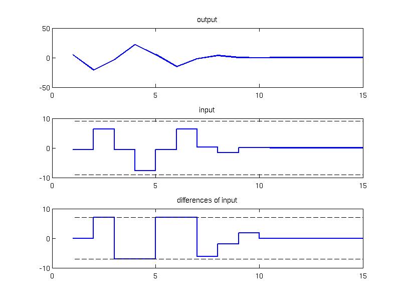
To add limits on the slew rate for the input, the deltaMin and deltaMax filters are activated and specified as {$ -10 \le \Delta u_k \le 10 $}

model.u.with('deltaMin');
model.u.with('deltaMax');
model.u.deltaMin = -7;
model.u.deltaMax = 7;

The penalties are provided as quadratic functions on the states and inputs

model.y.penalty = QuadFunction( 10 );
model.u.penalty = QuadFunction( 0.1 );

The online controller is constructed with the horizon 10

ctrl = MPCController(model, 10);

The ClosedLoop object is created and simulated for 15 samples for the initial condition x0 = [-1; -2; 3] . Note that for {$\Delta u$} formulation it is required to provide initial condition for the inputs as well u0 = 0 which is achieved as follows

loop = ClosedLoop(ctrl, model);
x0 = [-1; -2; 3]; 
u0 = 0;
Nsim = 15;
data = loop.simulate(x0, Nsim, 'u.previous', u0)

In the figure below one can see the closed loop trajectories of the MPC subject to input rate constraints. The first subfigure corresponds to the output of the system, the second subplot represent the input (with constraints in dashed line) and the third subplot shows input rate (with constraints in dashed line).

 (:source lang=MATLAB -getcode:) 
subplot(3, 1, 1);
plot(1:Nsim, data.Y, 'linewidth', 2); title('output');

subplot(3, 1, 2); 
stairs(1:Nsim, data.U, 'linewidth', 2); title('input');
hold on; 
plot( 1:Nsim, model.u.min*ones(1,Nsim), 'k--', 1:Nsim, model.u.max*ones(1,Nsim), 'k--');

subplot(3, 1, 3);
stairs(1:Nsim, [u0, diff(data.U) ], 'linewidth', 2); title('differences of input'); 
hold on; 
plot( 1:Nsim, model.u.deltaMin*ones(1,Nsim), 'k--', 1:Nsim, model.u.deltaMax*ones(1,Nsim), 'k--');

The lower bound constraint on a system signal is activated using deltaMin filter. The constraint is given as {$ \Delta s_k \ge \text{deltaMin}, k=0,\ldots, N $} on the signal {$s$} where {$\Delta s_k = s_k - s_{k-1} $} is the rate of the signal.

The upper bound on a system signal, indicated by max filter, is activated by default. The constraint is imposed over the whole prediction horizon and is considered as hard constraint {$ s_k \le \text{max}, k=0,\ldots, N $} on the signal {$s$}.

The lower bound on a system signal is indicated by min filter. Similarly as the upper bound constraint, the filter is activated by default and the constraint is imposed over the whole prediction horizon {$ s_k \ge \text{min}, k=0,\ldots, N $} on the signal {$s$}.

The upper bound constraint on a signal rate can be activated using deltaMax filter. It is given as {$ \Delta s_k \le \text{deltaMax}, k=0,\ldots, N $} on the signal {$s$} where {$\Delta s_k = s_k - s_{k-1} $} is the rate of the signal.

The lower bound constraint on a system signal is activated using deltaMin filter. The constraint is given as {$ \Delta s_k \le \text{deltaMax}, k=0,\ldots, N $} on the signal {$s$} where {$\Delta s_k = s_k - s_{k-1} $} is the rate of the signal.

The upper bound on a system signal, indicated by max filter, is activated by default. The constraint is imposed over the whole prediction horizon and is considered as hard constraint.

The lower bound on a system signal is indicated by min filter. Similarly as the upper bound constraint, the filter is activated by default and the constraint is imposed over the whole prediction horizon.

Consider the following example

  model = LTISystem('A', 0.5, 'B', 1);
  model.u.min = -3;
  model.u.max = 3;

with the penalties on the system state and input

  model.u.penalty = QuadFunction( 0.5 );
  model.x.penalty = QuadFunction( 1 );

The objective is to reach the value of the state {$ x_N = 3 $} at the end of the prediction horizon. The equality constraint {$ x_N = 3 $} can be modeled as the Polyhedron object

 Tset = Polyhedron( 'Ae', 1, 'be', 3);

and added to the MPC design using the terminalSet filter

 model.x.with('terminalSet');
 model.x.terminalSet = Tset;

Constructing the MPCController object with horizon 5 and evaluating the open-loop response for the zero initial value one obtains the result

 ctrl = MPCController(model, 5); 
 [u, feasible, openloop ] = ctrl.evaluate(0)
openloop.X

ans =

         0    0.0018    0.0118    0.0746    0.4730    3.0000

One can observe that the desired terminal state has been achieved in five steps of the prediciton.

The terminal set constraint is activated using the terminalSet filter. The constraint is active on the signal at the end of the prediction horizon {$x_N \in P $} where {$P$} is the polyhedral set.

and the following penalties

  model.u.penalty = QuadFunction(eye(2));
  model.x.penalty = QuadFunction(eye(2));

@] The initial conditions will be restricted to the polyhedral set (:source lang=MATLAB -getcode:) [@

Formulating a finite horizon MPC optimization problem over horizon 4 and solving it explicitly

ctrl = MPCController(model, 4);

and the following penalties

  model.u.penalty = QuadFunction(eye(2));
  model.x.penalty = QuadFunction(eye(2));

@] In this case, the constraints on the states will be activated over the whole prediction horizon using the setConstraint filter (:source lang=MATLAB -getcode:) [@

The finite horizon MPC optimization problem is solved parametrically over the horizon 4

ctrl = MPCController(model, 4);

The initialSet filter activates polyhedral constraints on the initlal states {$x_0 \in P$} in the prediction. The constraints are useful when solving parametric optimization problem because it limits the exploration space for unbounded problems. This filter corresponds to MPT2 field sysStruct.Pbnd. As an example, consider the model of the form

The setConstraintSet filter activates polyhedral constraints over the whole prediction horizon {$x_k \in P, k=0, \ldots, N$} in the prediction. Consider the same model as in the previous example

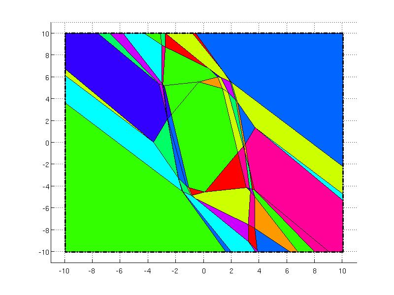
 model = LTISystem('A', [1.2 -0.8; 1.5 2.3], 'B', [0.5 -0.4; -1.2 0.8])

which operates under input constraints

 model.u.min = [-5; -4];
 model.u.max = [6; 3];

In this case, the constraints on the states will be activated over the whole prediction horizon using the setConstraint filter

P = Polyhedron('lb', [-10; -10], 'ub', [10; 10]);
model.x.with('setConstraint');
model.x.setConstraint = P;

The finite horizon MPC optimization problem is solved parametrically over the horizon 10

ctrl = MPCController(model, 10);
explicit_ctrl = ctrl.toExplicit()

The partition of the explicit controller is significantly smaller as in the previous example because the state constraints must be active over the whole horizon. The set constraints are depicted in the wired frame in the figure below.

explicit_ctrl.partition.plot()
hold on
P.plot('wire', true, 'linestyle', '-.', 'linewidth', 2)

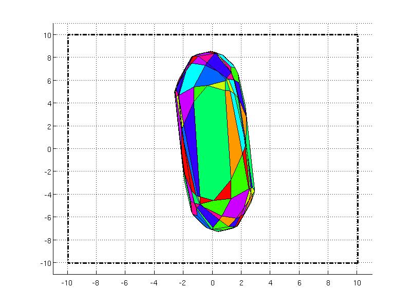
The initialSet filter activates polyhedral constraints on the initlal states {$x_0$} in the prediction. The constraints are useful when solving parametric optimization problem because it limits the exploration space for unbounded problems. This filter corresponds to MPT2 field sysStruct.Pbnd. As an example, consider the model of the form

 model = LTISystem('A', [1.2 -0.8; 1.5 2.3], 'B', [0.5 -0.4; -1.2 0.8])

which operates under input constraints

 model.u.min = [-5; -4];
 model.u.max = [6; 3];

The initial conditions will be restricted to the polyhedral set

P = Polyhedron('lb', [-10; -10], 'ub', [10; 10]);
model.x.with('initialSet');
model.x.initialSet = P;

Formulating a finite horizon MPC optimization problem over horizon 10 and solving it explicitly

ctrl = MPCController(model, 10);
explicit_ctrl = ctrl.toExplicit()

one can plot the resulting partition and the polyhedron set in wired frame to see that the solution is contained inside the initial constraint set.

explicit_ctrl.partition.plot()
hold on
P.plot('wire', true, 'linestyle', '-.', 'linewidth', 2)

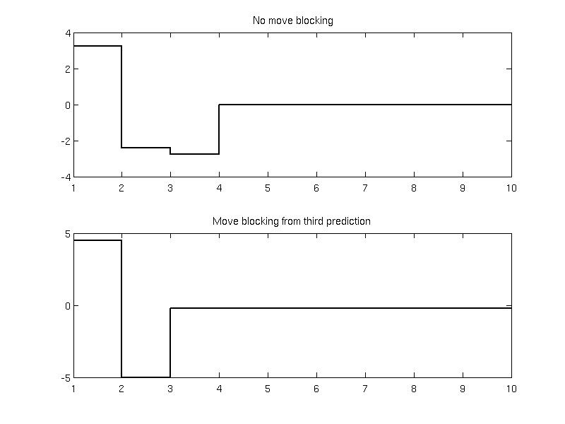
The move blocking constraint is activated using block filter. The move blocking constraint is useful for constraining the predicted control moves over the horizon to reduce the number of decision variables in the optimization problem. Consider a regulation problem of the following PWA model with a varying gain

 mode1 = LTISystem('A', [0.7 0.4; -1.3 0.9], 'B', [1.8; 0]);
 mode1.setDomain( 'x', Polyhedron( [1 0;-1 0], [5; 5]) );
 mode2 = LTISystem('A', [0.7 0.4; -1.3 0.9], 'B', [2.3; 0]);
 mode2.setDomain( 'x', Polyhedron( [-1 0], -5) )
 mode3 = LTISystem('A', [0.7 0.4; -1.3 0.9], 'B', [2.3; 0]);
 mode3.setDomain( 'x', Polyhedron( [1 0], -5) )
 model = PWASystem( [mode1, mode2, mode3] );

The model operates under state and input constraints

 model.x.min = [-20; -20]
 model.x.max = [20; 20];
 model.u.min = -5;
 model.u.max = 5;

For the MPC setup the following penalties are provided

 model.x.penalty = InfNormFunction( diag([0.5; 0.5]) );
 model.u.penalty = InfNormFunction( 1 );

and the online MPCController object is constructed with horizon N=10

 N = 10;
 complex_controller = MPCController(model, N);

To reduce the number of decision variables, the inputs from the third prediction step are constrained to be equal. This is achieved via the blocking constraint as follows

 model.u.with( 'block' );
 model.u.block.from = 3;
 model.u.block.to = N;
 simple_controller = MPCController(model, N);

To compare both controllers, the open-loop prediction is evaluated for the value of the state x0 = [-7, 8]:

x0 = [-7; 8];
[u1, feasible1, openloop1] = complex_controller.evaluate( x0 );
[u2, feasible2, openloop2] = simple_controller.evaluate( x0 );

and plotted

subplot(2, 1, 1); stairs(1:N, openloop1.U, 'linewidth', 2, 'color', 'k'); title(' No move blocking');
subplot(2, 1, 2); stairs(1:N, openloop2.U, 'linewidth', 2, 'color', 'k'); title(' Move blocking from third prediction ');

Any of the filters is activated using with method and deactivated by without method. The activation/deactivation must be done on a system signal such as inputs u, states x, and outputs y. For instance, consider activation of the terminal set constraint on the state variable. This is achieved by

model = LTISystem('A', 1, 'B', 1);
model.x.with('terminalSet')

The deactivation of the filter proceeds by

model.x.without('terminalSet')

In the next list you can find various filters for adjustment of MPC setups:

Adding binary constraints is achieved using the binary filter. To impose binary on all elements of a given variable use

model.u.binary = true;

To add binary only to elements indexed by idx, call

model.u.binary = idx;

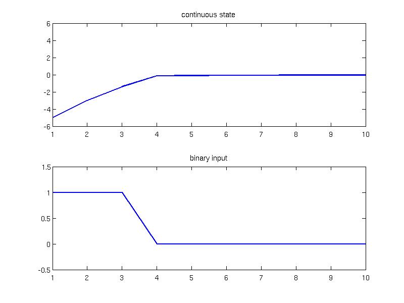
Consider the following example with one state and one binary input. The model is constructed and the binary filter is activated on the u signal

 model = LTISystem('A', 0.8, 'B', 1);
 model.u.with('binary')

In the rest of the MPC setup, the constraints are provided for the states

model.x.min = -5;
model.x.max = 5;

and penalties are specified

model.x.penalty = OneNormFunction( 1 );
model.u.penalty = OneNormFunction( 1 );

The online MPCController object is constructed with the horizon 5

horizon = 5;
ctrl = MPCController( model, horizon);

To verify that the binary constraints on input are respected, a closed loop simulation is performed from the initial condition x0 = -5 over 10 sampling instances:

 loop = ClosedLoop( ctrl, model);
 x0 = -5; 
 Nsim = 10;
 data = loop.simulate( x0, Nsim);

The simulation results are plotted and one can observe that the input provides only binary values

 subplot(2, 1, 1); plot( 1:Nsim, data.X(1:Nsim), 'linewidth', 2); title('continuous state'); axis([1 Nsim -6 6]);
 subplot(2, 1, 2); plot( 1:Nsim, data.U, 'linewidth', 2); title('binary input'); axis([1 Nsim -0.5 1.5]);

Filters on constraints specification

Binary constraint

Move blocking constraint

Initial set constraint

Set constraint

Terminal set constraint

Upper bound limit on a signal

Lower bound limit on a signal

Upper bound limit on a rate of a signal

Lower bound limit on a rate of a signal

Soft upper bound constraint

Soft lower bound constraint

Filters on penalties specification

Signal rate penalization

Signal rate penalization

Reference signal

Piecewise Affine penalty

Back to MPC synthesis overview.

Filters on system signals

• Filters on constraints specification
  • Binary constraint -- binary
  • Move blocking constraint -- block
  • Initial set constraint -- initialSet
  • Set constraint -- setConstraint
  • Terminal set constraint -- terminalSet
  • Upper bound limit on a signal -- max
  • Lower bound limit on a signal -- min
  • Upper bound limit on a rate of a signal -- deltaMax
  • Lower bound limit on a rate of a signal -- deltaMin
  • Soft upper bound constraint -- softMax
  • Soft lower bound constraint -- softMin
• Filters on penalties specification
  • Signal rate penalization -- deltaPenalty
  • Signal rate penalization -- terminalPenalty
  • Reference signal -- reference
  • Piecewise Affine penalty -- PWApenalty