• View
• Edit
• History
• Print

OperationsWithPolyhedra

Geometric operations with polyhedra

• Methods for determining basic properties
• Working with multiple polyhedra
• Geometric methods
  • Facet and vertex enumeration
  • Set containment
  • Chebyshev center
  • affineHull - affine hull
  • affineMap - affine maps
  • invAffineMap - inverse affine maps
  • grid - regular grid of the polytope
  • meshGrid - grid given as coordinates for 2D polytopes
  • mldivide - set difference
  • plus - Minkowski summation
  • minus - Pontryagin difference
  • normalize - normalization of H-representation
  • project - project a point onto a set
  • projection - orthogonal projection onto axis
  • slice - cuts of polyhedra
  • triangulate - triangulation
  • volume - computing a volume

For further help on the methods of the Polyhedron class, type help at the Matlab prompt. For instance, to obtain the help description for Minkowski summation in plus method, type

or display the Matlab documentation that contains additional examples on the geometric methods

and search for the specific method there.

Methods for determining basic properties

The Polyhedron class contains methods that are very useful for determining the basic properties such as

• emptyness - isEmptySet
• boundedness - isBounded
• full-dimensionality - isFullDim

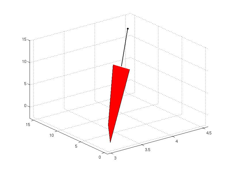
As an example, consider the lower-dimensional polyhedron in the dimension 3

To query, if the set is empty or nor, use

From the construction it is evident that the polyhedron is lower-dimensional because it contains one equality constraint. This fact can be checked using the method

Boundedness property can be queried by

method. One can plot the polyhedron to verify that the above properties are true

Working with multiple polyhedra

Polyhedra can be grouped into column or row arrays. For this purpose in MPT there exist overloaded horzcat and vertcat operators or [ ] brackets. Consider the two following polyhedra

The row array of polyhedra Q, R can be created twofold

Similarly, the column array is created as

Each polyhedron in the array can be extracted using indices, e.g.

Polyhedra in the array can be removed

The basic methods operate onto arrays

If the method cannot be executed on an array, the forEach function can be applied. For instance, to compute the grid function cannot be evaluated on an array and one observes an error

In this case, the forEach method can be applied that executes the function on each polyhedron in the array. For more help on forEach function type

The correct syntax for the above example using grid function is given as

To create a new copy of a Polyhedron object, or an array of polyhedra, the method copy must be invoked otherwise the new object point to the same data, i.e.

Geometric methods

Facet and vertex enumeration

The Polyhedron object can be created in two forms

• H-representation (by inequalities and equalities)

• V-representation (by vertices and rays)

which can be converted vice-versa. The conversion from H- to V-representation is achieved via computeVRep method. Consider the following polyhedron which is created in H-representation

To compute the V-representation, the method computeVRep method is called

To obtain the vertices and rays, one has to refer to V and R properties

Note that the method computeVRep is executed automatically when queried for vertices or rays using V or R properties.

The conversion from V- to H-representation is achieved via computeHRep method. Consider the following triangle

that comprises of three vertices. The H-representation can be computed by

and the facets can be extracted by pointing to H, He properties (or A, Ae, b, be)

When queried for facets, the method computeHRep is executed automatically. Note that conversion between H- and V-representations is numerically expensive and can become time-consuming for polyhedra with large number of facets or vertices. The numerical computation is delegated to an external CDD solver that should be present at the installation path. ( If not, type tbxmanager install cddmex to install it.)

Set containment

The Polyhedron class implements the contains method which tests whether a point (or a set of points) is contained inside a polyhedron. Consider the following polyhedron in V-representation

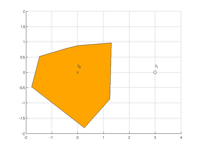
To test wheter the polyhedron P contains the origin x0 = [0; 0] , the function contains is invoked

The answer is yes, so the point {$x_0$} is contained inside the polyhedron. What about the point x1 = [3; 0] ?

The test containment for the points {$x_0$} and {$x_1$} is visualized in the figure below.

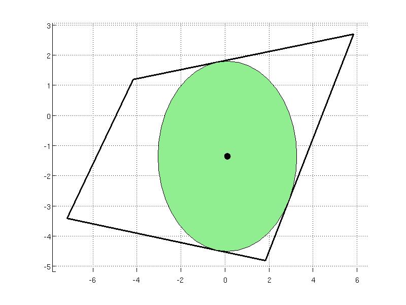
Chebyshev center

Computation of the Chebyshev center corresponds to inscribing the largest ball inside a polyhedron which is implemented in the chebyCenter method. The ball is described as {$ \{ x ~|~ \| x-x_c \|_2 \le r \} $} where {$x_c$} is the center of the ball and {$ r $} is the radius. Consider the following polyhedron

The data of the ball can be computed by calling

where the field x represents the center and r is the radius. The field exitflag is the status returned from the optimization solver. As the ball is a convex set, it can be represented as YSet object and plotted together with the polyhedron

Back to Computational Geometry overview.