Construction of functions over sets
This part explains construction of piecewise functions, i.e. functions defined over sets. To understand the basic concepts, you should be familiar with the construction of sets, constrution of unions of sets, and construction of functions.
- Single function over the set
- Piecewise Affine Function
- Piecewise Quadratic Function
- Piecewise Function
Single function over the set
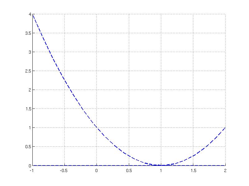
Function over the set can be constructed by attaching the Function object to an object derived from the ConvexSet class. Consider a quadratic function y = x^2 - 2*x +1 defined over the interval -1 <= x <= 2 . To represent such a function over the set in MPT, it is required to construct corresponding Function object and ConvexSet object and then add the function to the set using addFunction method:
S = Polyhedron('lb', -1, 'ub', 2);
S.addFunction(F,'alpha')
When adding the Function object to the ConvexSet object, it is required to provide the name of the function to be used for referencing. In the above example the quadratic function will be stored under the name "alpha". The name of the function is obligatory in order to distinguish multiple functions over the set. When the function has been attached, the object still behaves as a convex set and all methods applicable for ConvexSet class can be used, including additional methods for functions over sets. For instance, to plot the set one can use the plot method
that applies for objects derived from the ConvexSet class. To plot the function over the set, the specific method fplot applies
To plot both, the set and the function over the set, it is required to provide some arguments for the fplot method:
For more help on plotting functions over sets, type
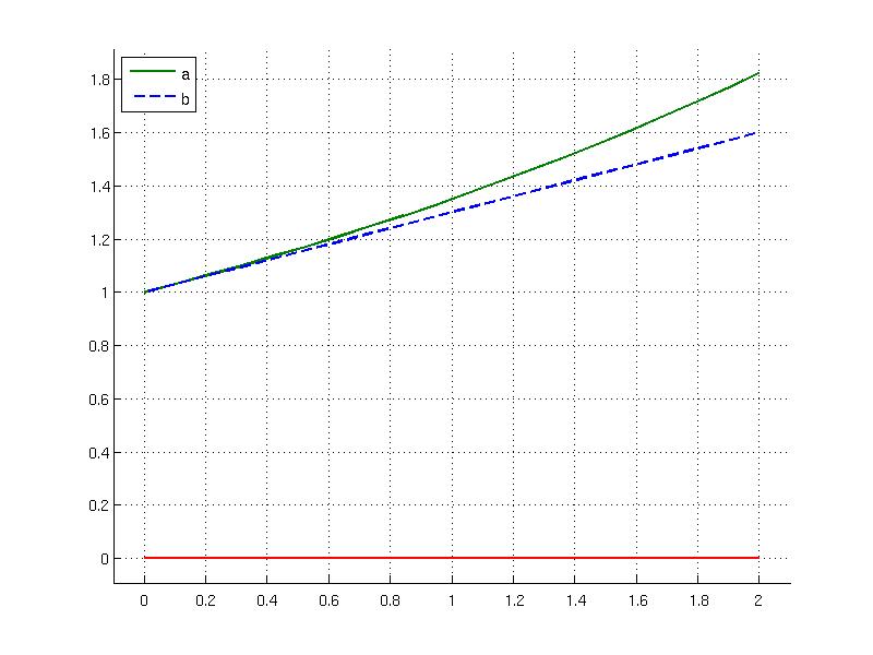
Multiple functions can be attached to a set. In the following example two functions are attached to an interval [0, 2]
f2 = AffFunction(0.3,1)
P = Polyhedron('lb', 0, 'ub', 2);
P.addFunction(f1, 'a')
P.addFunction(f2, 'b')
The stored function objects are accessible by index using the Func property or can be extracted via the getFunction method by pointing to their names
P.getFunction('b')
Referencing to the function name is useful for plotting the specific function over the set
hold on
P.fplot('b','color','blue', 'linewidth', 2, 'linestyle', '--');
P.plot('color', 'red', 'linewidth', 2)
legend(2,'a', 'b')
The evaluation of the function for a particular point is achieved via feval method and the function must be referenced by its name. For instance, to evaluate the function "a" for a point 0.5 can be done as follows
Piecewise Affine Function
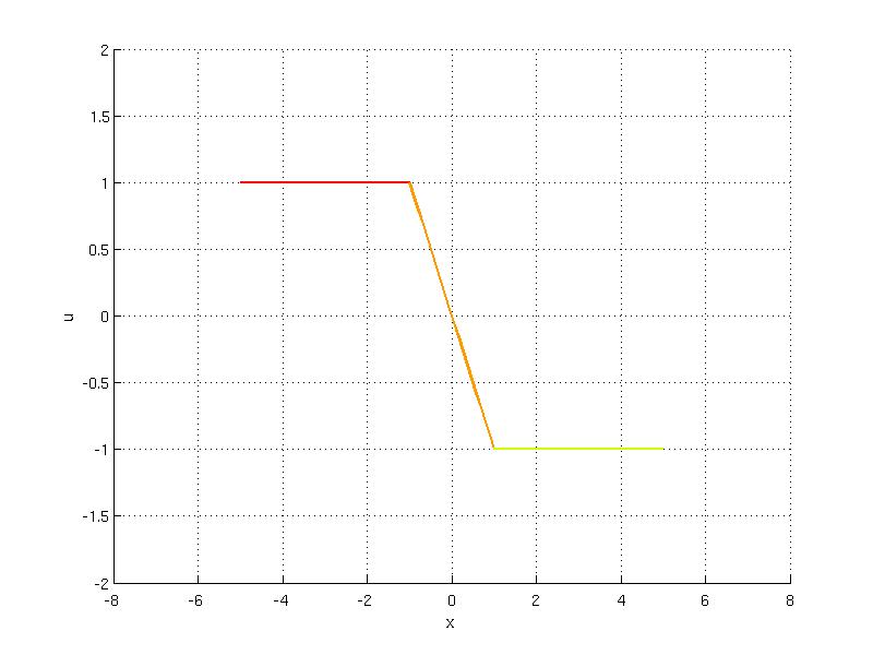
Piecewise affine (PWA) function can be represented as union of sets that have attached an affine function. In the previous section you can learn how to construct single function over a set. Merging multiple affine functions over sets to a compact form of the PolyUnion object represents a piecewise affine function over polyhedra. As an example, consider a saturated controller u(x) = 1 if -5 <= x<= -1, u(x) = -x if -1 <= x <= 1, u(x) = -1 if 1 <= x <= 5 . To create PWA function the corresponding intervals are defined as Polyhedron objects:
R(2) = Polyhedron('lb', -1, 'ub', 1);
R(3) = Polyhedron('lb', 1, 'ub', 5);
Secondly, the function objects are created and attached to the intervals under the same name
f(2) = AffFunction(-1);
f(3) = AffFunction(0, -1);
R(1).addFunction(f(1), 'u');
R(2).addFunction(f(2), 'u');
R(3).addFunction(f(3), 'u');
Thirdly, the functions over sets are merged to a single PolyUnion object. If some properties of the union are known at the time of constructing the PolyUnion object, one can associate them directly to the constructor:
The PWA function can be plotted using overloaded fplot function that applies for PolyUnion objects:
axis([-8 8 -2 2])
xlabel('x')
ylabel('u')
Evaluation of PWA functions proceeds via overloaded feval function. If there is only one function attached to a set, one does not have to refer to the name
Note that for two points -1,1 there exist two functions values because these points lie at the connection of the intervals. When evaluation of PWA function is invoked for such a point, two values are returned
U.feval(1)
To get rid of multiple values, it is always recommended to use the extended evaluation syntax that considers the tie-break criterion to decide which value to use. For instance, if an anonymous function @(x)0 is used as a tie-breaking function, it takes always the first choice
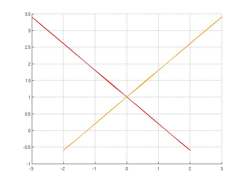
Consider a PWA function that is defined over two regions which are overlapping.
P(1).addFunction( AffFunction(-0.8, 1), 'a' );
P(2) = Polyhedron('lb', -2, 'ub', 3);
P(2).addFunction( AffFunction(0.8, 1), 'a' );
U = PolyUnion('Set', P, 'Overlaps', true)
U.fplot()
Note that evaluation of such a function could return two different values for a point that is shared in two intervals. This case can be resolved by a tie-breaking function which in this example takes the minimum of the same function 'a'
U.feval(-1, 'a', 'tiebreak', 'a')
Piecewise Quadratic Function
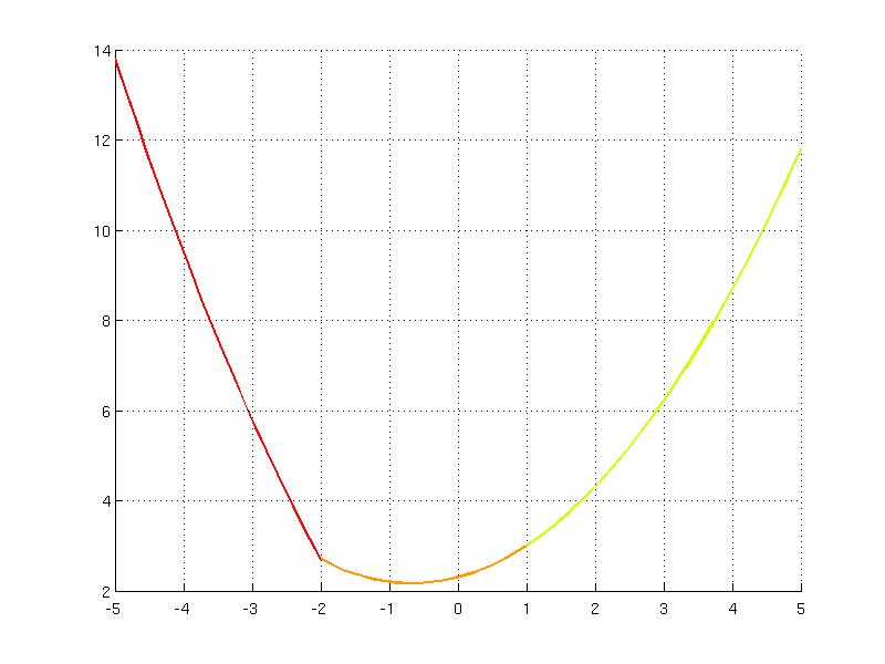
Piecewise quadratic (PWQ) function can be represented as an union of quadratic functions over polyhedra. Consider the following function y(x) = 0.3*|x-1|^2 + |x+2| over the interval [-5, 5]. The function can be decomposed to three intervals:
y1 = 0.3*x^2 - 1.6*x - 1.7 if [-5, -2]y2 = 0.3*x^2 + 0.4*x + 2.3 if [-2, 1]y3 = 0.3*x^2 + 0.4*x + 2.3 if [1, 5]
where the two intervals share the same function value. Such a function can be modeled in MPT with the help of Polyhedron, QuadFunction and PolyUnion objects:
S(1).addFunction( QuadFunction(0.3, -1.6, -1.7), 'q' );
S(2) = Polyhedron('lb', -2, 'ub', 1);
S(2).addFunction( QuadFunction(0.3, 0.4, 2.3), 'q' );
S(3) = Polyhedron('lb', 1, 'ub', 5);
S(3).addFunction( QuadFunction(0.3, 0.4, 2.3), 'q' );
U = PolyUnion('Set', S, 'Overlaps', false, 'Convex', true, 'FullDim', true, 'Bounded', true)
U.fplot()
Evaluation of PWQ function is achieved using the overloaded feval method as for PWA functions:
Piecewise Function
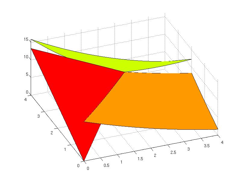
The piecewise function represents any general function defined over polyhedra. Consider the following partition comprising of three regions in two-dimensional space:
P(2) = Polyhedron([0 0; 4 0; 4 2; 2 2]);
P(3) = Polyhedron([0 4; 4 4; 4 2; 2 2]);
To each of the polyhedra a function is assigned under the same name "g", then the PolyUnion object is created and the function over the union is plotted.
P(1).addFunction(F1, 'g');
F2 = QuadFunction(0.2*eye(2), [-3.2, 2.9], 11.2);
P(2).addFunction(F2, 'g');
F3 = Function(@(x) 0.4*x(1)^2 + 0.8*sqrt(x(1)+x(2)) - 1.3*x(1)*x(2) + 14.2 );
P(3).addFunction(F3, 'g');
U = PolyUnion('Set', P, 'Overlaps', false, 'Convex', true)
U.fplot()
Back to computational geometry overview.