OperationsWithSets
Geometry.OperationsWithSets History
Hide minor edits - Show changes to markup
b = [1.72 3.84 3.05 0.03];
b = [1.72; 3.84; 3.05; 0.03];
Extreme point in a given dimension
Extreme point in a given direction
Outer approximation
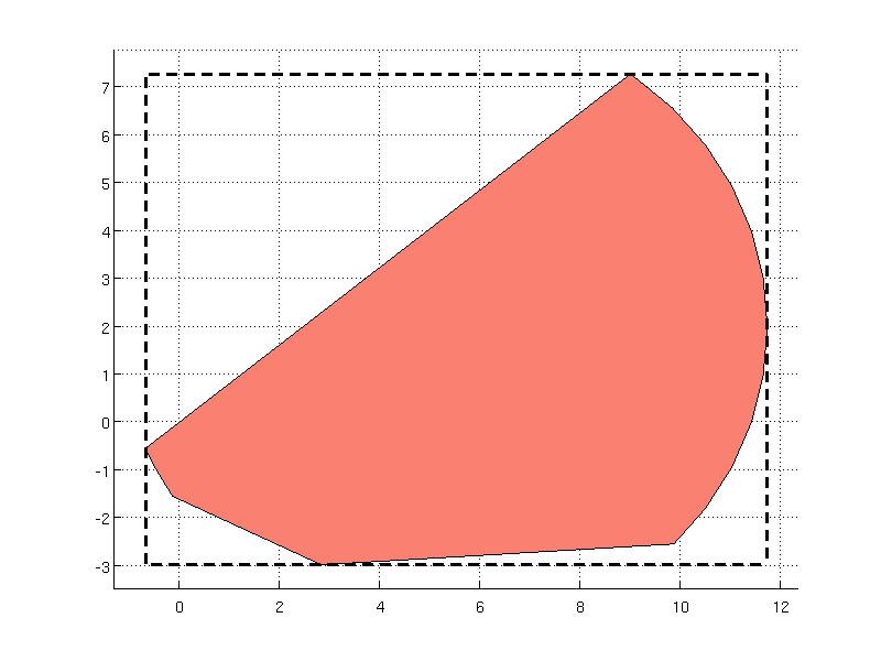
Computation of the bounding box over the set is implemented in outerApprox method:
B = S.outerApprox()
The method returns a polyhedron with lower and upper bounds that are stored internally and can be accessed by referring to Internal property
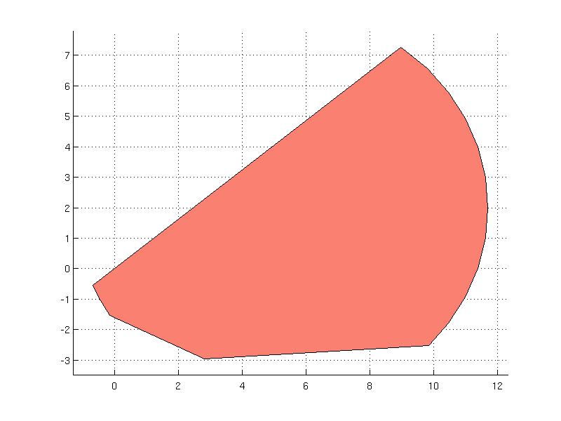
B.Internal.lb

ans =

   -0.6775
   -2.9647

B.Internal.ub

ans =

   11.6969
    7.2648
Comparison of the bounding box B wih the orignal set S can be found on the figure below which was generated with the following command:
 S.plot('color', 'salmon');
 hold on
 B.plot('wire', true, 'linestyle', '--', 'linewidth', 2)
 hold off
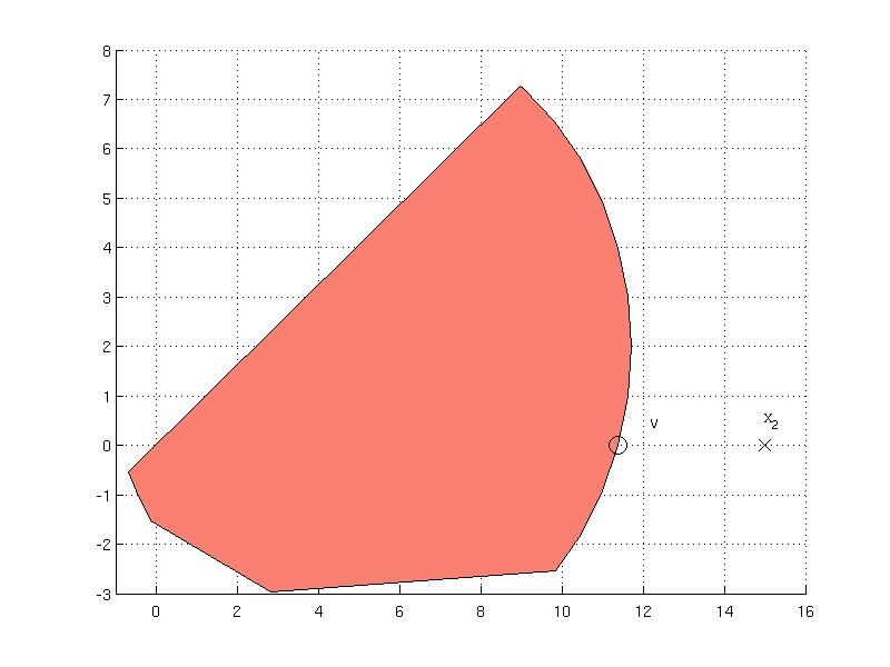
The ray-shooting problem is given by { max alpha s.t. alpha*x in Set } and is available in the shoot method. As an example, consider computation of the maximum of the set for the point x2 = [15; 0]
The ray-shooting problem is given by { max alpha s.t. alpha*x in Set } and is available in the shoot method. As an example, consider computation of the maximum of the set in the direction of the point x2 = [15; 0] which gives the value of alpha
 alpha = S.shoot( x2 )

 alpha =

    0.7586
Multiplying this value with the point x2 one obtains the point v = alpha * x2 that lies on the boundary of the set
 v = alpha * x2

 v =

   11.3788
         0
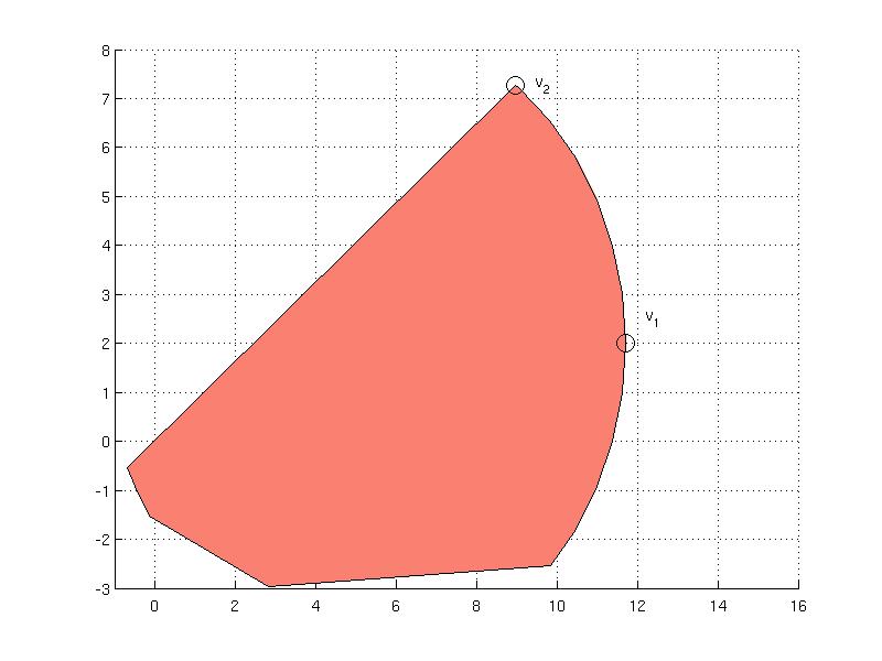
One can visually inspect the location of the computed extreme points v1 and v2 in the figure below:
One can visually inspect the location of the computed extreme points v1.x and v2.x in the figure below:
Computing a support of the set in a given direction
For a given point x, the support of a set is given as { max x'*y s.t. y in Set }. This feature is implemented in the support method. The syntax of the support method requires a point x which determines the direction and the value of the maximum over the set is returned.
S.support(x3)

ans =

   36.3241
Note that computation of the support is available also in the extreme method.
Maximum over the set in a given direction - ray shooting
The ray-shooting problem is given by { max alpha s.t. alpha*x in Set } and is available in the shoot method. As an example, consider computation of the maximum of the set for the point x2 = [15; 0]
Extreme point in a given dimension
Computation of extreme points for a convex set is implemented in the extreme method. The method accepts a point as an argument that specifies the direction in which to compute the extreme point. For instance, for the point x2, the extreme method results in
 v1 = S.extreme( x2 )

v1 =

    exitflag: 1
         how: 'Successfully solved (SeDuMi-1.3)'
           x: [2x1 double]
        supp: 175.4535
The output variable v1 contains the status returned from the optimization solver in exitflag and how fields. The extreme point is stored in x variable and the field supp corresponds to a support of the set given as { max x'*y s.t. y in Set }. The extreme point in the direction x3 = [0; 5] is given as
 x3 = [0; 5];
 v2 = S.extreme( x3 )

 v2 =

    exitflag: 1
         how: 'Successfully solved (SeDuMi-1.3)'
           x: [2x1 double]
        supp: 36.3241
One can visually inspect the location of the computed extreme points v1 and v2 in the figure below:
The YSet object implements a method for computing a separation hyperplane from a point which is accessed as separate method.
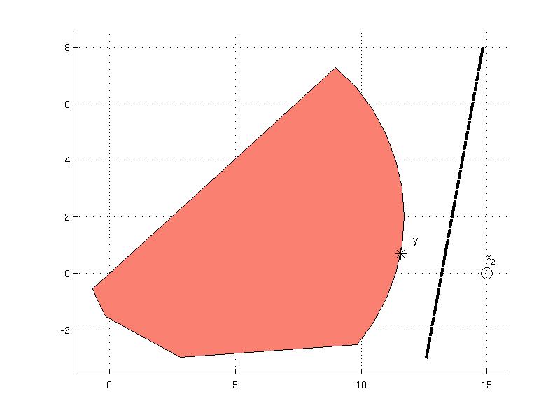
The YSet object implements the separate method that computes a hyperplane that separates the set from a given point. As an example, consider computation of a separating hyperplane from the set S and the point x2:
 He = S.separate(x2)

 He  =

  -3.4346    0.7044  -45.3730
which returns a data corresponding to a hyperplane equation { x | He*[x; -1] = 0 }. To plot the computed hyperplane, a Polyhedron object is constructed
P = Polyhedron('He', He)
and plotted.
Projection of a point to a set
Point projection onto a set
Distance to the point
Distance to a point
Projection of a point to a set
Computation of the distance is achieved also in the project method which computes the closest point to the set. For the point x2 the projection operation results in a structure with four fields
 res = S.project(x2)

 res =

    exitflag: 1
         how: 'Successfully solved (SeDuMi-1.3)'
           x: [2x1 double]
        dist: 3.5061
The field exitflag informs about the status returned from the optimization solver which can be found also in the how field. The closed point is computed in x field and the value about the distance can be found in dist field. One can verify that the computed point by the projection operation is the same as by distance operation
 res.x

ans =

   11.5654
    0.7044
Separation hyperplane from a point
The YSet object implements a method for computing a separation hyperplane from a point which is accessed as separate method.
but the point x2 = [12; 0] lies not:
but the point x2 = [15; 0] lies not:
x2 = [12; 0];
x2 = [15; 0];
Computing distance from the set to a given point is achieved using distance method. For instance, the distance to the point x2 that lies outside of the set S can be computed as follows
 data = S.distance(x2)

ans =

    exitflag: 1
        dist: 0.5932
           x: [2x1 double]
           y: [2x1 double]
The output from the method is a structure with four fields indicating the result of the computing the distance. The field exitflag indicates the exit status from the optimization solver, the actual distance is available in dist field and fields x, y indicate the coordinates of the two points for which the distance has been computed. It can be extracted from the field y which point is the closest to the point x2 and plotted.
data.y

ans =

   11.5654
    0.7044

This set will be used next to demonstrate some methods that can be applied to YSet objects.
Set containment test
To check if the point is contained in the set or not, there exist a method contains. For instance, the point x1=[8; 0] lies in the set
x1 = [8; 0];
S.contains(x1)

ans =

     1
but the point x2 = [12; 0] lies not:
x2 = [12; 0];
S.contains( x2 )

ans =

     0

Geometric operatioins with convex sets
Geometric operations with convex sets
The ConvexSet class offers a couple of methods for use in computational geometry. Consider a following set which is created as an intersection of quadratic and linear constraints
 x = sdpvar(2, 1);
 A = [-0.46 -0.03; 0.08 -1.23; -0.92 -1.9; -1.92  2.37];
 b = [1.72 3.84 3.05 0.03];
 constraints = [ 0.2*x'*x-[2.1 0.8]*x<=2; A*x<=b ];
 S = YSet(x, constraints);
which is plotted in salmon color
(:source lang=MATLAB -getcode:)
S.plot('color', 'salmon')
Working with multiple sets
To create a new copy of the ConvexSet, the copy must be employed, otherwise the new object points to the same data stored in the original object
If the sets are stored in an array, some methods can operate on the array, for instance
Snew = S.copy()
row_array1.isBounded() column_array2.isEmptySet()
If the method is not applicable on the array, it can be invoked for each element in the array using forEach method:
statement = row_array1.forEach(@isBounded)
The forEach method is a fast replacement of for-loop and it can be useful for user-specific operations over an array of convex sets.
To create a new copy of the ConvexSet, the copy must be employed, otherwise the new object points to the same data stored in the original object
Snew = S.copy()
(:comment Note that in general, when constructing a set with nonlinear constraints, an appropriate nonlinear optimization solver needs to be present. Typically, if you have Optimization Toolbox installed on your Matlab distribution, then the problem is passed to FMINCON solver. :)
(:comment Note that in general, when constructing a set with nonlinear constraints, an appropriate nonlinear optimization solver needs to be present. Typically, if you have Optimization Toolbox installed on your Matlab distribution, then the problem is passed to FMINCON solver. :)
(:comment
:)
(:comment Note that in general, when constructing a set with nonlinear constraints, an appropriate nonlinear optimization solver needs to be present. Typically, if you have Optimization Toolbox installed on your Matlab distribution, then the problem is passed to FMINCON solver. :)
To create a new copy of the ConvexSet, the copy must be employed, otherwise the new object points to the same data stored in the original object
Snew = S.copy()
 z = sdpvar;
 t = sdpvar;
 constraints1 = [ z^2 - 5*t <= 1 ;   0 <= t <= 1 ];
 S = YSet( [z; t], constraints1);
 constraints2 = [ z^2 + 5*t <= 1 ;   0 <= t <= 1 ];
 R = YSet( [z; t], constraints2);
which are plotted in different colors
(:source lang=MATLAB -getcode:)plot(S, 'color', 'lightgreen', R, 'color', 'yellow')
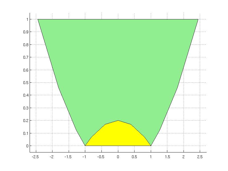
Note that in general, when constructing a set with nonlinear constraints, an appropriate nonlinear optimization solver needs to be present. Typically, if you have Optimization Toolbox installed on your Matlab distribution, then the problem is passed to FMINCON solver.
The above sets can be concatenated into an array using overloaded [ ] operators. The column concatenation can be done using brackets or vertcat method which are equivalent:
column_array1 = [S; R]
column_array2 = vertcat(S, R)
The row concatenation using brackets or horzcat method
row_array1 = [S, R]
row_array2 = horzcat(S, R)
To create a new copy of the ConvexSet, the copy must be employed, otherwise the new object points to the same data stored in the original object
Snew = S.copy()
Determining basic properties of the YSet object
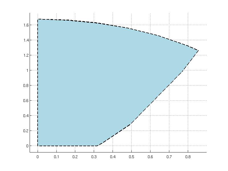
Consider the following example where the set is build from nonlinear constraints
Methods for determining basic properties of sets
Consider the following example where the set is built from the following constraints
constraints = [ 0 <= x <= 5; 4*x(1)^2 - 2*x(2) >= 0.4; sqrt( x(1)^2 + 0.6*x(2)^2 ) <= 1.3 ];
constraints = [ 0 <= x <= 5; 4*x(1)^2 - 2*x(2) <= 0.4; sqrt( x(1)^2 + 0.6*x(2)^2 ) <= 1.3 ];
(:comment Note that in general, when constructing a set with nonlinear constraints, an appropriate nonlinear optimization solver needs to be present. Typically, if you have Optimization Toolbox installed on your Matlab distribution, then the problem is passed to FMINCON solver. :)
Note that plotting of general convex sets could become time consuming because the set is sampled with an uniform grid. The value of the grid can be changed using the grid option of the plot method, for details type
help ConvexSet/plot
To create a new copy of the ConvexSet, the copy must be employed, otherwise the new object points to the same data stored in the original object
Snew = S.copy()
S.isEmptySet
S.isEmptySet()
Another useful property is boundedness which can be checked using the isBounded method, i.e.
S.isBounded()
These properties can be veriefied by plotting the set using plot method
S.plot('color', 'lightblue', 'linewidth', 2, 'linestyle', '--')
Geometric operatioins with convex sets
Determining basic properties of the YSet object
Consider the following example where the set is build from nonlinear constraints
(:source lang=MATLAB -getcode:)x = sdpvar(2, 1); constraints = [ 0 <= x <= 5; 4*x(1)^2 - 2*x(2) >= 0.4; sqrt( x(1)^2 + 0.6*x(2)^2 ) <= 1.3 ]; S = YSet(x, constraints);
It is very often of interest to check wheter the set is empty or not. In MPT there exist an isEmptySet method that checks whether the set is empty
S.isEmptySet
Geometric methods
Back to Computational Geometry overview.